Week 5: 09/03/23

Table of Contents

Comments on Problem sheet A2

Question 2

Most of the answers for this question got most of the parts correct. For a lot of the solutions I got I put “what about $\mu=0$?” This might seem like a minor detail but if you put $\mu>0$ and $\mu<0$ for your conditions then you should state separately what happens for $\mu=0$. Also, reason you should look at this case is because, for $\mu=0$, $x^*=0$ and $f’(0)=0$. This means that it is a non-hyperbolic steady state so we actually can’t tell from the linear stability analysis whether it is stable or unstable. This is as far as you are expected to go although the written solutions do go into more detail if you are interested.

Question 4

In my opinion, the easiest way to do part (a) was to leave everything in terms of $x,y$ until the end. Again I won’t put in the details here since they are in the written solutions if you want to see them. Anyway, we end up finding that $\kappa=\mu-\lambda$.

The steady states of this are then $p^*=0,1$. From here we can use our linear stability analysis: $$ \frac{df}{dp} = \kappa(1-2p) $$ and substitute in our steady states for both $\kappa>0$ and $\kappa<0$.

At this point I think it’s important to look back at the question and think about what is going on in the system and what the question is really asking. The thing I wanted you to say once you’d found the stability of these points was that if:

• $\kappa>0$: $\mu>\lambda$, so species $x$ grows exponentially faster than $y$ and eventually dominates as $p\rightarrow 1$ as $t\rightarrow\infty$ (as long as $p_0\neq 0$).
• $\kappa<0$: $\mu<\lambda$, so species $y$ grows exponentially faster than $x$ and eventually dominates as $p\rightarrow 0$ as $t\rightarrow\infty$ (as long as $p_0\neq 1$).

Finally, many of you said that for $\kappa=0$, the steady states $p^*=0,1$ are non-hyperbolic so nothing can be said. This is kind of true but also not. Yes the linear stability tells us $f’(p^*)=0$ but we can still say things about the system without using linear stability.

$$ \kappa=0 \Rightarrow f(p) = 0, \quad \forall p $$ This means that $p=p^*, \forall p$ (all values of p are steady states). This means that the proportion of bacteria species stays the same no matter the initial condition. Now, this makes sense since $\kappa=0$ implies $\mu=\lambda$ so they grow at the same rate. Again this is as far as you were expected to go but I added an extra question if you got this far asking what this means for the stability of these steady states.

Look back at the definitions of stability and asymptotic stability. The colloquial interpretations of these terms were

• Stable: starts near, stays near.
• Asymptotically stable: starts near, tends to eventually.

Which of these apply to the case where $\kappa=0$? Well if we start at $p_0$ we stay there and if we start at $p_0+\varepsilon$ where $\varepsilon$ is a small positive constant we stay at $p_0+\varepsilon$ too. We can see, therefore, that $p_0$ is stable but is not asymptotically stable because trajectories near it never actually move towards it. I think this is a good example of how the two definitions are distinct even though in many of the situations we see, the stable points are also asymptotically stable and vice-versa.

Outline of lecture content

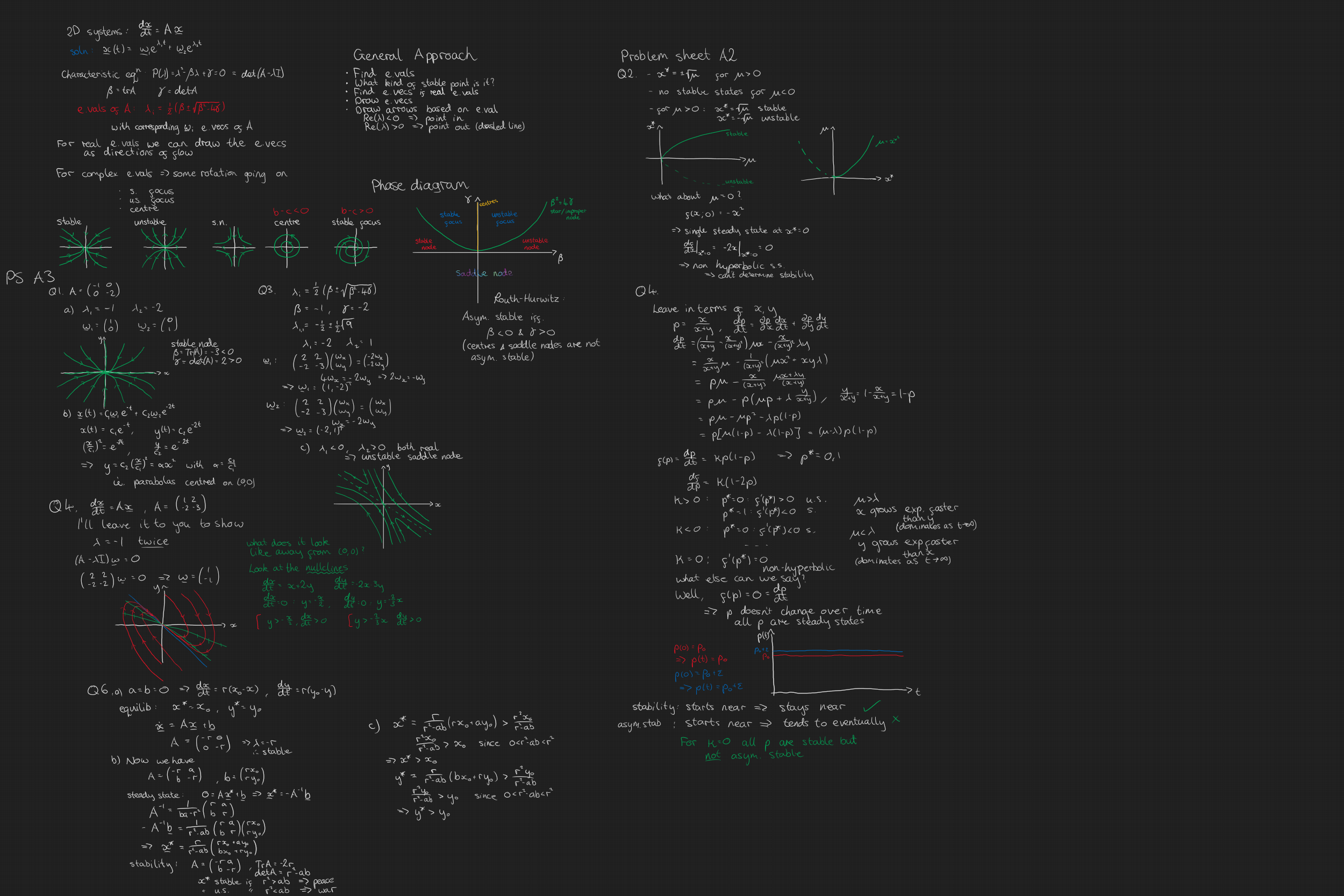
The main concept introduced last week was expanding what we’ve done to linear systems of ODEs. You spent a lot of time last semester solving these kinds of systems but now, just like with the 1D systems we’ve studied, we want to quickly understand the behaviour of the system quickly without solving it explicitly.

The notes go through the different situations we can have for 2D linear systems and below I’ve put a diagram of all of these situations. As in the notes we have $$ \frac{d\mathbf{x}}{dt} = A\mathbf{x}, \quad \mathbf{x} \in \mathbb{R}^2, A\in \mathbb{R}^{2\times2} $$ and we denote $\mathrm{Tr}(A)=\gamma$, $\mathrm{det}(A)=\beta$

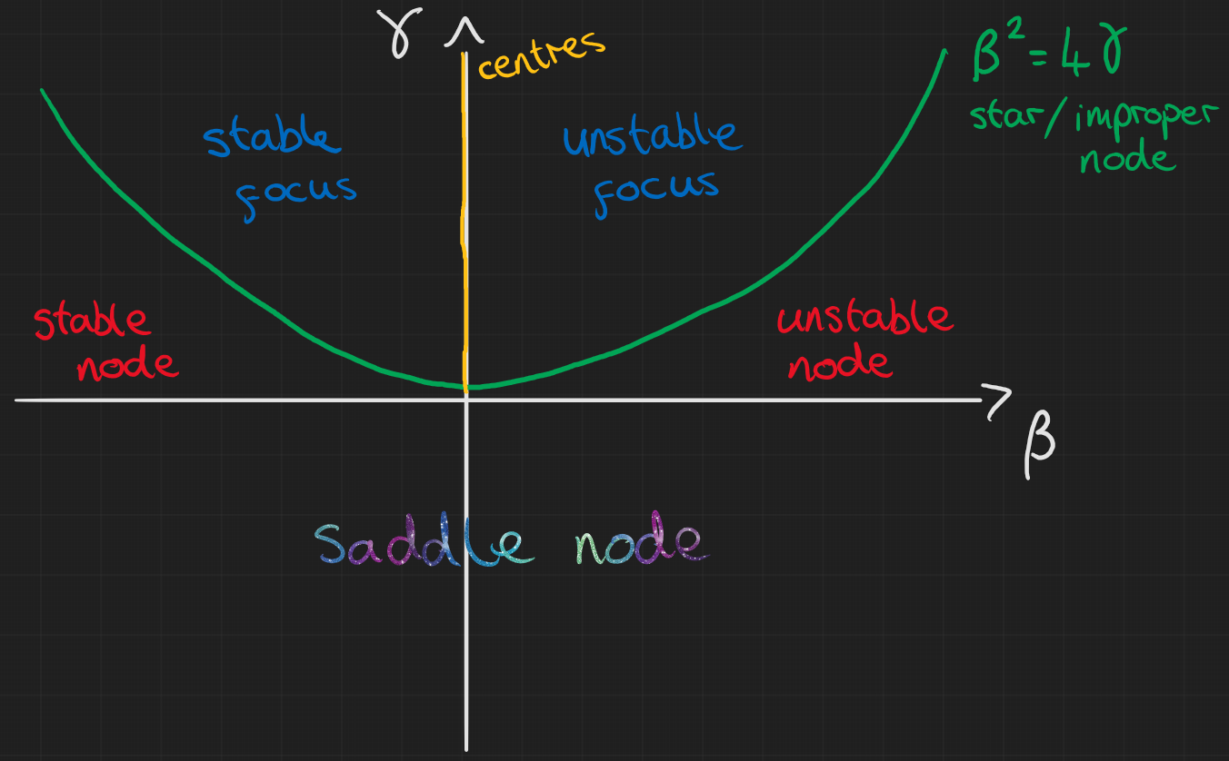
Example diagrams of these situations can be found in the notes but I have most of them in the notes linked at the top of this page. Also, below I’ve put a video of how these phases go from one type of node to the other. On the left is an example of what the trajectories might look like for the $\gamma,\beta$ values shown in the figure on the right.

Problem sheet A3

Question 1

Question 2

Question 3

Question 4