Table of Contents
Problem sheet 1
The main point of most of this module is to test your abilities to turn a problem often in the form of a paragraph into a mathematical model which you then solve and then learn something about the behaviour of the system or whatever from the solution. Because of this I will not just give you the start of the problem because that is often half of the difficulty in the question. Learning how to do this quickly and effectively now will help you a lot later down the road, so do keep trying even if you feel stuck.
Question 1
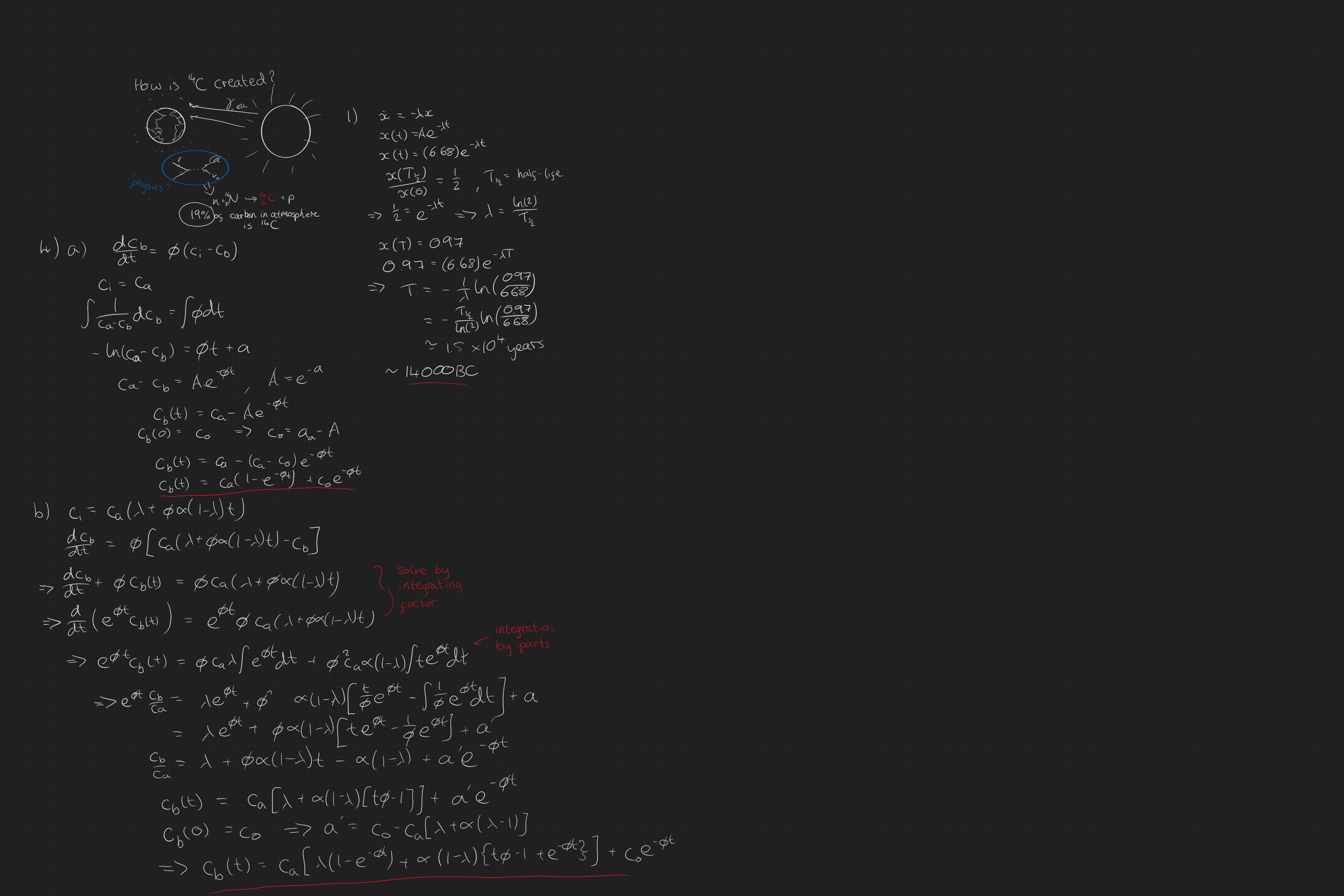
One question you might ask about this problem is why does the dead plant matter have a decreasing number of radioactive carbon atoms but the carbon in the atmosphere does not? This is a bit of a side note but essentially Carbon-14 is produced when particles in the upper atmosphere and troposphere collide with cosmic particles and all sorts of interesting physics happens. These interactions sometimes produce neutrons which can then collide with the abundand nitrogen in the air to make Carbon-14 with the following interaction:
147N + n → 146C + p
Anyway the point is that once the plant dies it is separated from this system of radioactive carbon being created and decaying so we just have the decay. From the lectures we saw that the general radioactive decay equation is $$\dot{x}(t) = -\lambda x(t)$$ which has the solution $$x(t) = x(0)e^{-\lambda t} .$$ The key is to figure out what this rate of decay $\lambda$ is in terms of the half-life which we are given. The half-life is the time, $T_{1/2}$ for the amount of 14C to half so we can write that $$ \frac{1}{2} = \exp\left[-\lambda T_{1/2}\right]$$ which rearranges to give $$ \lambda = \frac{\ln(2)}{T_{1/2}}.$$ From here, all we need to do is recognise that we want to find the time $T$ where the activity is $0.97$ and we know that initially the activity was $6.68$ so we have $$ 0.97 = 6.68 e^{-\lambda T}.$$ With some more rearranging we get the solution $$ T = \frac{T_{1/2}}{\ln(2)}\ln\left(6.68/0.97\right) \approx 1.5951 \times 10^4 \text{ years}$$
Wondered why the radioactive decay is what it is? It may make intuitive sense to you or it may not. Either way a nice way to think about it is that the probability of a single atom decaying in time $t$ is an exponentially distributed random variable with rate parameter $\lambda$. Over a period of time $t$ the probability that is has not decayed is $1-F(t)=1-e^{-\lambda t}$, where $F(t)$ is the cumulative distribution. If all of the atoms can be treated as independent (and as long as the number of particles is large) then the expected number of particles left by time t is $\langle N\rangle = N_0 e^{-\lambda t}$.
Or we could say that rate of one atom decaying is $\lambda$ so the rate of any of the $N$ particles decaying is $N\lambda$ so this gives us an instantaneous rate of change of the system so $dN=-N\lambda dt$.
I’m sure given some more thought, one of you could make this a bit more rigourous.
Question 2
Should be relatively straight forward
Question 3
- a) What do the two terms on the RHS mean physically?
- b) What does the steady state distribution mean for the ODE?
- c) This one is just a following through the maths so I’ll leave that up to you.
Question 4
This question is pretty straight forwards in terms of setting up the problem. All we need to do is solve the ODE in the case that $c_i=c_a=\text{ constant}$ and substitute in the initial condition that the concentration starts at some value $c_0=c(0)$ so we can substitute this condition in for any constants of integration. Then we do the same for the second case.
The trick in part b is to notice that we can rewrite the ODE as $$ \begin{aligned} c_b’(t) & = \phi \left( c_a \left( \lambda + \phi \alpha (1-\lambda) t \right)- c_b(t)\right) \\\ c_b’(t) + \phi c_b(t) & = \phi\left(c_a\left(\lambda+\phi\alpha(1-\lambda)t\right)\right) \\\ \frac{d}{dt}\left\{c_b(t)e^{\phi t}\right\} & = e^{\phi t}\phi\left(c_a\left(\lambda+\phi\alpha(1-\lambda)t\right)\right) \end{aligned} $$ where we’ve used an integrating factor. From here we can integrate both sides and use integration by parts for the $t\exp[\phi t]$ term.
Jeremy Worsfold
Postdoctoral Fellow
My research interests include Collective Behaviour, speficially swarming models and interacting particles Systems. I also have interests in Reinforcement Learning and Scientific Computing.